Note
Go to the end to download the full example code.
Visualizing & Evaluating OoD Detection algorithms#
Hint
We recommend reading Inferring with Confidence first.
In this tutorial, we use the
Visualization & Evaluation in Classification API from scio.eval to
compare several confidence score algorithms in a classification setup,
both visually and quantitatively.
Let’s start with preparing a trained model and some InD calibration data. These should be naturally defined by your own use-case. For this tutorial, we use a lightweight Tiniest architecture trained on CIFAR10 and hosted on our hub, and fetch the corresponding calibration data from our HuggingFace dataset, not seen during training.
# These should be defined by your use-case
import torch
from datasets import load_dataset  # type: ignore[import-untyped, unused-ignore]

calib_set = load_dataset("ego-thales/cifar10", name="calibration")["unique_split"]
calib_data, calib_labels, _ = calib_set.with_format("torch")[:].values()
calib_data = calib_data / 255  # Convert [0, 255] uint8 from HuggingFace to [0, 1] float

sample_shape = calib_data.shape[1:]
net = torch.hub.load("ThalesGroup/scio:hub", "tiniest", trust_repo=True, verbose=False)
net = net.to(calib_data)
/home/docs/checkouts/readthedocs.org/user_builds/sciortd/checkouts/latest/.venv/lib/python3.14/site-packages/multiprocess/connection.py:335: SyntaxWarning: 'return' in a 'finally' block
  return f
/home/docs/checkouts/readthedocs.org/user_builds/sciortd/checkouts/latest/.venv/lib/python3.14/site-packages/multiprocess/connection.py:337: SyntaxWarning: 'return' in a 'finally' block
  return self._get_more_data(ov, maxsize)
1. Configure algorithms to compare#
Let use choose, say \(3\) confidence score algorithms from
those implemented in
scio.scores. We will compare them to the
Softmax baseline. We arbitrarily choose
GradNorm, Gram and
KNN. Each algorithm requires defining which
internal representations it will analyze. Some authors may recommend
the use of specific layers, while others propose general approaches
free of choosing (e.g. Gram). Let us identify
layers to select.
from scio.recorder import Recorder

Recorder(net, input_data=calib_data[[0]])  # Visualize layers
Recorder instance for the following network
============================================================================================================================================
Layer (type (var_name):depth-idx)        Input Shape               Output Shape              Param #                   Param %
============================================================================================================================================
Tiniest (Tiniest)                        [1, 3, 32, 32]            [1, 10]                   --                             --
├─Conv2d (conv1): 1-1                    [1, 3, 32, 32]            [1, 48, 32, 32]           1,344                       1.38%
├─LayerNorm2d (ln1): 1-2                 [1, 48, 32, 32]           [1, 48, 32, 32]           --                             --
│    └─LayerNorm (ln): 2-1               [1, 32, 32, 48]           [1, 32, 32, 48]           96                          0.10%
├─Block (l1): 1-3                        [1, 48, 32, 32]           [1, 48, 32, 32]           48                          0.05%
│    └─Conv2d (dwconv1): 2-2             [1, 12, 32, 32]           [1, 12, 32, 32]           120                         0.12%
│    └─Conv2d (dwconv2): 2-3             [1, 12, 32, 32]           [1, 12, 32, 32]           600                         0.62%
│    └─Conv2d (dwconv3): 2-4             [1, 12, 32, 32]           [1, 12, 32, 32]           600                         0.62%
│    └─LayerNorm2d (ln): 2-5             [1, 48, 32, 32]           [1, 48, 32, 32]           --                             --
│    │    └─LayerNorm (ln): 3-1          [1, 32, 32, 48]           [1, 32, 32, 48]           96                          0.10%
│    └─Conv2d (fc1): 2-6                 [1, 48, 32, 32]           [1, 96, 32, 32]           4,704                       4.82%
│    └─Conv2d (fc2): 2-7                 [1, 48, 32, 32]           [1, 48, 32, 32]           2,352                       2.41%
├─Block (l2): 1-4                        [1, 48, 32, 32]           [1, 48, 32, 32]           48                          0.05%
│    └─Conv2d (dwconv1): 2-8             [1, 12, 32, 32]           [1, 12, 32, 32]           120                         0.12%
│    └─Conv2d (dwconv2): 2-9             [1, 12, 32, 32]           [1, 12, 32, 32]           600                         0.62%
│    └─Conv2d (dwconv3): 2-10            [1, 12, 32, 32]           [1, 12, 32, 32]           600                         0.62%
│    └─LayerNorm2d (ln): 2-11            [1, 48, 32, 32]           [1, 48, 32, 32]           --                             --
│    │    └─LayerNorm (ln): 3-2          [1, 32, 32, 48]           [1, 32, 32, 48]           96                          0.10%
│    └─Conv2d (fc1): 2-12                [1, 48, 32, 32]           [1, 96, 32, 32]           4,704                       4.82%
│    └─Conv2d (fc2): 2-13                [1, 48, 32, 32]           [1, 48, 32, 32]           2,352                       2.41%
├─Block (l3): 1-5                        [1, 48, 32, 32]           [1, 48, 32, 32]           48                          0.05%
│    └─Conv2d (dwconv1): 2-14            [1, 12, 32, 32]           [1, 12, 32, 32]           120                         0.12%
│    └─Conv2d (dwconv2): 2-15            [1, 12, 32, 32]           [1, 12, 32, 32]           600                         0.62%
│    └─Conv2d (dwconv3): 2-16            [1, 12, 32, 32]           [1, 12, 32, 32]           600                         0.62%
│    └─LayerNorm2d (ln): 2-17            [1, 48, 32, 32]           [1, 48, 32, 32]           --                             --
│    │    └─LayerNorm (ln): 3-3          [1, 32, 32, 48]           [1, 32, 32, 48]           96                          0.10%
│    └─Conv2d (fc1): 2-18                [1, 48, 32, 32]           [1, 96, 32, 32]           4,704                       4.82%
│    └─Conv2d (fc2): 2-19                [1, 48, 32, 32]           [1, 48, 32, 32]           2,352                       2.41%
├─Conv2d (dsconv): 1-6                   [1, 48, 32, 32]           [1, 80, 16, 16]           3,920                       4.02%
├─LayerNorm2d (ln2): 1-7                 [1, 80, 16, 16]           [1, 80, 16, 16]           --                             --
│    └─LayerNorm (ln): 2-20              [1, 16, 16, 80]           [1, 16, 16, 80]           160                         0.16%
├─Block (l4): 1-8                        [1, 80, 16, 16]           [1, 80, 16, 16]           80                          0.08%
│    └─Conv2d (dwconv1): 2-21            [1, 20, 16, 16]           [1, 20, 16, 16]           200                         0.21%
│    └─Conv2d (dwconv2): 2-22            [1, 20, 16, 16]           [1, 20, 16, 16]           1,000                       1.03%
│    └─Conv2d (dwconv3): 2-23            [1, 20, 16, 16]           [1, 20, 16, 16]           1,000                       1.03%
│    └─LayerNorm2d (ln): 2-24            [1, 80, 16, 16]           [1, 80, 16, 16]           --                             --
│    │    └─LayerNorm (ln): 3-4          [1, 16, 16, 80]           [1, 16, 16, 80]           160                         0.16%
│    └─Conv2d (fc1): 2-25                [1, 80, 16, 16]           [1, 160, 16, 16]          12,960                     13.29%
│    └─Conv2d (fc2): 2-26                [1, 80, 16, 16]           [1, 80, 16, 16]           6,480                       6.64%
├─Block (l5): 1-9                        [1, 80, 16, 16]           [1, 80, 16, 16]           80                          0.08%
│    └─Conv2d (dwconv1): 2-27            [1, 20, 16, 16]           [1, 20, 16, 16]           200                         0.21%
│    └─Conv2d (dwconv2): 2-28            [1, 20, 16, 16]           [1, 20, 16, 16]           1,000                       1.03%
│    └─Conv2d (dwconv3): 2-29            [1, 20, 16, 16]           [1, 20, 16, 16]           1,000                       1.03%
│    └─LayerNorm2d (ln): 2-30            [1, 80, 16, 16]           [1, 80, 16, 16]           --                             --
│    │    └─LayerNorm (ln): 3-5          [1, 16, 16, 80]           [1, 16, 16, 80]           160                         0.16%
│    └─Conv2d (fc1): 2-31                [1, 80, 16, 16]           [1, 160, 16, 16]          12,960                     13.29%
│    └─Conv2d (fc2): 2-32                [1, 80, 16, 16]           [1, 80, 16, 16]           6,480                       6.64%
├─Block (l6): 1-10                       [1, 80, 16, 16]           [1, 80, 16, 16]           80                          0.08%
│    └─Conv2d (dwconv1): 2-33            [1, 20, 16, 16]           [1, 20, 16, 16]           200                         0.21%
│    └─Conv2d (dwconv2): 2-34            [1, 20, 16, 16]           [1, 20, 16, 16]           1,000                       1.03%
│    └─Conv2d (dwconv3): 2-35            [1, 20, 16, 16]           [1, 20, 16, 16]           1,000                       1.03%
│    └─LayerNorm2d (ln): 2-36            [1, 80, 16, 16]           [1, 80, 16, 16]           --                             --
│    │    └─LayerNorm (ln): 3-6          [1, 16, 16, 80]           [1, 16, 16, 80]           160                         0.16%
│    └─Conv2d (fc1): 2-37                [1, 80, 16, 16]           [1, 160, 16, 16]          12,960                     13.29%
│    └─Conv2d (fc2): 2-38                [1, 80, 16, 16]           [1, 80, 16, 16]           6,480                       6.64%
├─AdaptiveAvgPool2d (avgpool): 1-11      [1, 80, 16, 16]           [1, 80, 1, 1]             --                             --
├─Linear (fc): 1-12                      [1, 80]                   [1, 10]                   810                         0.83%
============================================================================================================================================
Total params: 97,530
Trainable params: 97,530
Non-trainable params: 0
Total mult-adds (Units.MEGABYTES): 44.73
============================================================================================================================================
Input size (MB): 0.01
Forward/backward pass size (MB): 9.05
Params size (MB): 0.39
Estimated Total Size (MB): 9.45
============================================================================================================================================
Currently recording: None
============================================================================================================================================
BLOCK3 = (1, 5)
FEATURE_MAPS = (1, 11)
LOGITS = (1, 12)
Now we configure our algorithms, using default or standard parameters,
and the somewhat arbitrarily identified layers for
Gram. See
Implementing your own OoD Detection algorithm to use your own
algorithm!
from scio.scores import GradNorm, Gram, KNN, Softmax

scores_and_layers = (  # type: ignore[var-annotated]
    (Softmax(), []),
    (GradNorm(), [LOGITS]),
    (Gram(), [BLOCK3, FEATURE_MAPS, LOGITS]),
    (KNN(k=int(len(calib_data) ** 0.4)), [FEATURE_MAPS]),
)
2. Prepare score functions#
With fit_scores(), we can now easily calibrate the
algorithms.
from scio.eval import fit_scores

scores_fit = fit_scores(scores_and_layers, net, calib_data, calib_labels)
0:00:11 Fitting Scores... (1000 samples) ━━━━━━━━━━━━━━━━━━━━━━━━━━━━━━ 4/4 Done
3. Define InD and OoD scenarios#
For evaluation, our InD scenario is naturally defined as the CIFAR10 test data. We only use \(1\,000\) random samples out of the \(10\,000\) available.
test_set = load_dataset("ego-thales/cifar10", name="test")["unique_split"]
ind = test_set.with_format("torch").shuffle()[:1000]["image"] / 255
As for OoD, we arbitrarily use vertical flips, darker images and uniformly random samples.
oods_title = ("Vertical flip", "Darker", "Uniformly random")
oods = (ind.flip(2), ind * 0.5, torch.rand_like(ind))
4. Compute confidence scores on scenarios#
We can easily compute confidence scores for all the prepared scenarios
with compute_confidence().
from scio.eval import compute_confidence

confs_ind, confs_oods = compute_confidence(
    scores_fit,
    ind=ind,
    oods=oods,
    oods_title=oods_title,
)
0:01:31 Computing confidences... ━━━━━━━━━━━━━━━━━━━━━━━━━━━━━━━━━━━━━━ 4/4 Done
5. Visualize the results#
Now, we simply use summary_plot() to visualize the
results.
from matplotlib import rcParams

from scio.eval import summary_plot

rcParams["figure.figsize"] = (15, 9)  # Adjust tutorial layout
summary_plot(
    confs_ind,
    confs_oods,
    scores_and_layers=scores_and_layers,
    oods_title=oods_title,
)
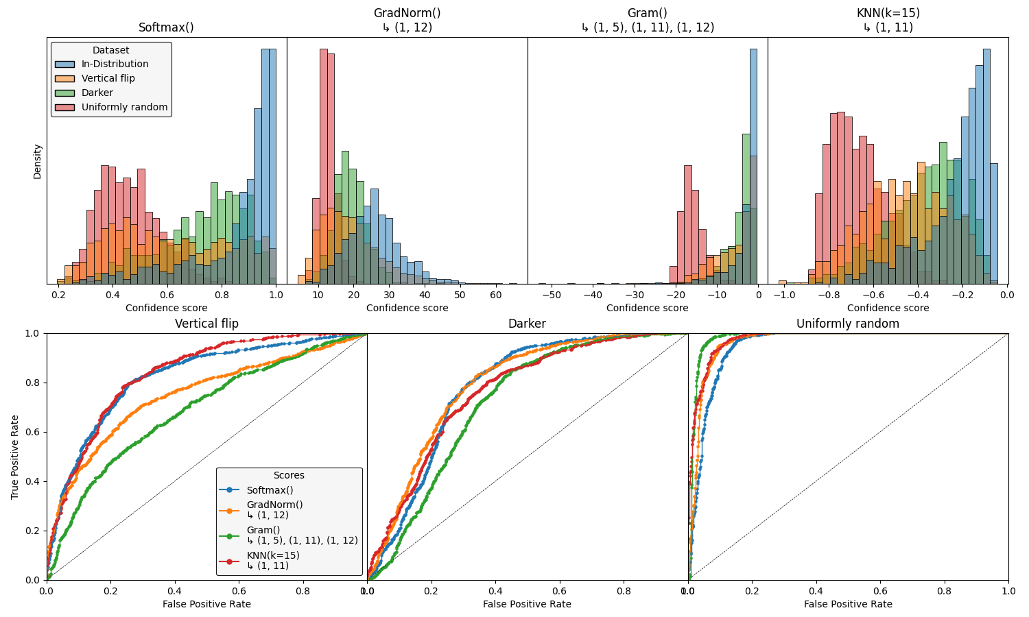
The first row shows the confidence scores distributions, one graph per scores function. Colors inside a given graph represent different scenarios: InD, Vertical flip, Darker and Uniformly random.
The second row shows the ROC curves for the OoD Detection task (which is in fine a binary classification task). There is one graph per InD/OoD pair, so \(3\) graphs here. In each graph, colors represent score functions: Softmax, GradNorm, Gram and KNN.
This visualization provides very insightful details for experienced users. The next section will help with quantifying these results.
Important
Confidence scores evaluation characterizes the ability to identify OoD samples based on the confidence scores associated with the predictions of the model. It provides no information regarding the correctness of the predictions themselves.
6. Define metrics to get quantified results#
In scio.eval, we implemented a few standard
Discriminative Power metrics. Let us choose \(2\) for our
tutorial: a partial AUC and
TPR\(@ 5\%\). See
Implementing your own Discriminative Power metric to use your
own metric.
Using compute_metrics() and
summary_table(), we get quantitative results from our
confidence scores.
from scio.eval import AUC, TPR, compute_metrics, summary_table

metrics = (AUC(max_fpr=0.2), TPR(max_fpr=0.05))
evals = compute_metrics(confs_ind, confs_oods, metrics)
summary_table(
    evals,
    scores_and_layers=scores_and_layers,
    oods_title=oods_title,
    metrics=metrics,
)
            Evaluation of 4 scores against 3 OoD sets and 2 metrics:
                      AUC(max_fpr=0.2) / TPR(max_fpr=0.05)
┏━━━━━━━━━━━━━━━━━━━━━━━━━━━┳━━━━━━━━━━━━━━━┳━━━━━━━━━━━━━━━┳━━━━━━━━━━━━━━━━━━┓
┃ Scores                    ┃    OoD 1:     ┃    OoD 2:     ┃      OoD 3:      ┃
┃ ↳ Recorded layers         ┃ Vertical flip ┃    Darker     ┃ Uniformly random ┃
┡━━━━━━━━━━━━━━━━━━━━━━━━━━━╇━━━━━━━━━━━━━━━╇━━━━━━━━━━━━━━━╇━━━━━━━━━━━━━━━━━━┩
│ Softmax()                 │ 0.452 / 0.350 │ 0.223 / 0.114 │  0.738 / 0.612   │
├───────────────────────────┼───────────────┼───────────────┼──────────────────┤
│ GradNorm()                │ 0.404 / 0.332 │ 0.291 / 0.141 │  0.813 / 0.808   │
│ ↳ (1, 12)                 │               │               │                  │
├───────────────────────────┼───────────────┼───────────────┼──────────────────┤
│ Gram()                    │               │               │                  │
│ ↳ (1, 5), (1, 11), (1,    │ 0.276 / 0.174 │ 0.158 / 0.049 │  0.894 / 0.946   │
│ 12)                       │               │               │                  │
├───────────────────────────┼───────────────┼───────────────┼──────────────────┤
│ KNN(k=15)                 │ 0.445 / 0.314 │ 0.277 / 0.157 │  0.865 / 0.807   │
│ ↳ (1, 11)                 │               │               │                  │
╰───────────────────────────┴───────────────┴───────────────┴──────────────────╯
In each cell, the \(2\) values correspond to the \(2\) chosen
metrics. Locally, you can also use the baseline option in
summary_table() for advanced CLI highlighting.
7. Be lazy#
For good measure, we mention that summary() directly
performs the summary_plot(),
compute_metrics() and
summary_table() calls described above, at once!
[Bonus] Profiling#
Let us compare the execution times of our \(4\) algorithms
(including the baseline) using the
timer attribute presented in
Inferring with Confidence.
for score, _ in scores_and_layers:
    score.timer.report  # Report execution times
    print("----")
        ScoreTimer report for
  Softmax(act_norm=None, mode='raw')
          at 0x701f9de5e510
┏━━━━━━━━━━━━━┳━━━━━━━━━━━┳━━━━━━━━━━┓
┃  Operation  ┃ # samples ┃ Duration ┃
┡━━━━━━━━━━━━━╇━━━━━━━━━━━╇━━━━━━━━━━┩
│  inference  │      1000 │ 4.911 s  │
│  inference  │      1000 │ 4.878 s  │
│  inference  │      1000 │ 4.858 s  │
│  inference  │      1000 │ 4.900 s  │
│ calibration │      1000 │ 4.710 μs │
╰─────────────┴───────────┴──────────╯
  Entries are listed from newest to
                oldest
----
        ScoreTimer report for
       GradNorm(act_norm=None,
  discard_functional_forward=False,
      grad_norm=1.0, mode='raw',
           temperature=1.0)
          at 0x701f9de5e900
┏━━━━━━━━━━━━━┳━━━━━━━━━━━┳━━━━━━━━━━┓
┃  Operation  ┃ # samples ┃ Duration ┃
┡━━━━━━━━━━━━━╇━━━━━━━━━━━╇━━━━━━━━━━┩
│  inference  │      1000 │ 5.439 s  │
│  inference  │      1000 │ 5.464 s  │
│  inference  │      1000 │ 5.399 s  │
│  inference  │      1000 │ 10.41 s  │
│ calibration │      1000 │ 3.640 μs │
╰─────────────┴───────────┴──────────╯
  Entries are listed from newest to
                oldest
----
        ScoreTimer report for
         Gram(act_norm=None,
  calib_labels='pred', cut_off=0.1,
    max_gram_order=8, mode='raw',
       separate_diagonal=False)
          at 0x701f9de5d010
┏━━━━━━━━━━━━━┳━━━━━━━━━━━┳━━━━━━━━━━┓
┃  Operation  ┃ # samples ┃ Duration ┃
┡━━━━━━━━━━━━━╇━━━━━━━━━━━╇━━━━━━━━━━┩
│  inference  │      1000 │ 6.269 s  │
│  inference  │      1000 │ 6.307 s  │
│  inference  │      1000 │ 6.298 s  │
│  inference  │      1000 │ 6.324 s  │
│ calibration │      1000 │ 6.456 s  │
╰─────────────┴───────────┴──────────╯
  Entries are listed from newest to
                oldest
----
        ScoreTimer report for
 KNN(act_norm=2.0, index_metric='l2',
          k=15, mode='raw')
          at 0x701f9cc24550
┏━━━━━━━━━━━━━┳━━━━━━━━━━━┳━━━━━━━━━━┓
┃  Operation  ┃ # samples ┃ Duration ┃
┡━━━━━━━━━━━━━╇━━━━━━━━━━━╇━━━━━━━━━━┩
│  inference  │      1000 │ 5.023 s  │
│  inference  │      1000 │ 4.996 s  │
│  inference  │      1000 │ 5.008 s  │
│  inference  │      1000 │ 5.011 s  │
│ calibration │      1000 │ 4.899 s  │
╰─────────────┴───────────┴──────────╯
  Entries are listed from newest to
                oldest
----
These facilitate overhead computation and provide decisive information when choosing an algorithm for a time-sensitive use-case.
Total running time of the script: (2 minutes 5.769 seconds)